Introduction
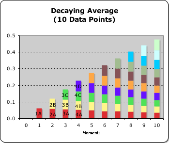
The prior article provided introductions and definitions for a variety of terms associated with the Living Algorithm System. We found that the Living Average can be broken into Events (the horizontal component) and Moments (the vertical component). When both of these components are visualized simultaneously, the graphic result is a grid of colored rectangles. We refer to these colored rectangles as quanta of info energy and to the entire graph as the Living Average Grid. Now that we have defined our terms algebraically we can begin our derivations. Our express purpose in this article is to derive the values or dimensions of the info quanta in the Living Average Grid.
Searching for Content (Data) Based Equations for the Info Quanta
1. Let's start our proof with the basic Living Algorithm. This is the algebraic expression for the famous Living Average, the Living Algorithm's 1st derivative.
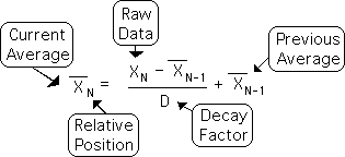
As noted, the X without a hat represents the Raw Data, while the Xs with hats are Living Averages, one the Current Average, the other the Previous Average. The subscript N indicates the Relative Position of each X in their respective data stream. If N equals 1, the X is the first element and so on.
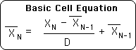
2. As indicated by the equation, the Current Living Average is a function of the Raw Data and the Previous Living Average only. The Previous Living Average is a composite measure because we need to know other facts to determine its value. Because the Present is based upon the immediate Past, this equation is contextual.
![]()
The general form for this expression reveals everything anyone might want to know about the dynamics of the present moment. Tied up so completely in the context of the Moment, this composite measure reveals nothing about past history. Content is buried in Context. The only way we can derive the dimensions of our info quanta is to dig into the Context to find the hidden Content.
3. To fulfill this quest, we must derive the content-based equations that are buried in the Living Algorithm. In other words we seek algebraic expressions that are based completely in the Raw Data that makes up the data stream. In the case of this article, our purpose is to derive an equation that determines the Current Living Average based upon the Raw Data only. Instead of including composite measures, the Living Average would be expressed as a function of the Raw Data.
![]()
This equation is content-based. In other words, the Living Algorithm measure, the Living Average in this case, is expressed in terms of the data alone. Deriving this equation is the focus of this proof. Understanding the features of this equation will enable us to determine the height of the color rectangles, our quanta of information.
The Content-based Equation for the Living Average at the 1st Moment
4. Let us start simple. What does the basic Living Algorithm tell us about the data stream's first Living Average – the Living Average at the first moment?
N = 1 for the data stream's first Living Average. Plugging in the appropriate values in the general equation:
![]()
5. Because this is the first Living Average, the Prior Living Average is assumed to be 0.
![]()
6. The Prior Living Average drops out of the equation and we are left with this simple expression - the initial Raw Data divided by the Decay Factor. This is the content-based equation for the first Living Average.
![]()
That derivation was easy. How about the 2nd Living Average – the Living Average at the 2nd moment?
Defining K, the Scaling Factor
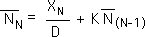
7. Before proceeding forth, let us introduce a useful algebraic simplification, also employed in previous works. The following algebraic expression is another version of the Living Algorithm's Living Average. In words, the Raw Data is shrunk by a factor of D and the Previous (or Past) Average is scaled by a factor of (D-1)/D. These two values are then added together to determine the Current Average.
![]()
8. For ease of expression, let us call K the value for the Scaling Factor. Note that K will always be less than 1, as D-1 is always less than D.
![]()
9. This is the simplified equation that we will employ.
![]()
The Content-based Equation for the Living Average
10. The following is the context-based equation for the 2nd Living Average (N=2).
![]()
11. We already know the value of the 1st Living Average (Equation 6). When we plug this value in the equation, this is the result.
![]()
This is the content-based equation for the 2nd Living Average.
12. The following equation is the context-based equation for the 3rd Living Average (N=3).
![]()
13. We plug in the content-based value for the 2nd Living Average (Equation 11) into the equation and multiply through by K. This gives us the content-based equation for the 3rd Living Average.
![]()
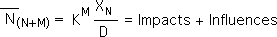
14. Employing the same reasoning, we arrive at the general content-based equation for the Living Average, when N could be any number.
![]()
General Ramifications of the Content-based Equation for the Living Average
There are a few points of note. First, the general equation is additive or accumulative. There are no negatives. Second, the impact of each byte of raw data fades with time. With each repetition (iteration) of the Living Algorithm process, the impact of the data on the total Living Average is scaled back by a factor of K. Third, we are not sure what the equation has to say about the size of the color rectangles, the individual info quanta. To uncover this value, we must expand our perspective to include Events.
The Sum of Events = the Living Average
Graph
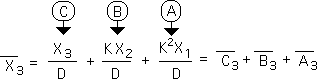
15. Let's look at the graph again. It is evident from the visual presentation that the sum of each of the color rectangles (the info quanta) in the numbered columns yields the total Living Average at that moment. This notion is reflected in the following equation (Eq. 0.3).
![]()
In words, the Living Average, XN bar, at any point is determined by the sum of the Events appropriate to that particular Moment. For instance, the Living Average for the 3rd moment (N=3) is the sum of the Living Averages of Events A, B, and C at the 3rd moment.
This same reasoning applies to all the data stream derivatives, including the Active Pulse's Directional. As an example, the Directional (the Living Algorithm's 2nd derivative) at the 5th moment (N=5) equals the sum of the Living Averages of Events A, B, C, D, and E at the 5th moment.
Algebraic Expressions for Impacts & Influences in the Living Average Grid
Now that we have established the algebraic terminology, let us continue our search for the dimensions of our info quanta, the colored rectangles.
Partial Derivatives
At the beginning of a general Event N, the Living Algorithm digests XN to create a fresh family of partial derivatives (rates of change), including a partial Living Average. Each of these derivatives is associated with Event N. We refer to these measures as partial because they are added to other partial measures to obtain the total measure.
16. We refer to the initial partial Living Average of Event N as NN bar. N bar refers to the event that is spawned, while N the subscript refers to the position in the data stream. With each successive moment the position in the data stream changes, but the Event remains the same. We determine the value of this partial Living Average in the normal fashion. Diminish the data byte, XN, by a factor of D. Then add this value to the previous Living Average, which has been scaled, K N(N-1) bar.
17. However, NN bar is the first Living Average of Event N by definition. There is no prior Living Average. In other words the value of NN-1 bar is 0.
18. The final term drops out of Equation 16. The value of the 1st Living Average of any event, N, always equals the data byte, XN, that spawns the event divided by D, the Decay Factor. This value is the height of the first info quanta of every Event in the Living Average Grid. Remember we defined an Event's first moment as an Impact - the instant impact of the entering Data upon the Living Average (or any other Living Algorithm derivative). This is indicated in the equation below.
19. Let's see what happens to the 2nd moment (N+1) in Event N. We apply the Living Algorithm to get the following equation.
20. However, Event N is based upon the data point that spawned it, XN. No more raw data enters its stream, by definition. In other words, all subsequent data equals zero (XN+N = 0)
21. The first term on the right side of the equation drops out. This leaves us with the scaled prior Living Average. But we know the content-based value of this term (Equation 18). We substitute this value to obtain the following result.
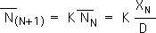
In other words, the same algebraic expression reveals the 2nd value of any Living Average Event. It is always the initial raw data that spawned the Event, XN, divided by D and scaled by K. This is always true. No exceptions. This value is independent of any prior data in the stream.
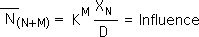
22. We can apply the same reasoning to come up with a general term for all subsequent values in the Event. Because there is no more data added to this mini-system, each subsequent value is merely scaled again (multiplied by K.) This leads to the following equation. Simply speaking each repetition (iteration) of the Living Algorithm process scales (K) the prior value in the Event. Nothing more or less. As shown in the graph, the colored rectangles become increasingly smaller. We defined the first moment of an Event as an Impact. We defined the subsequent moments in the Event as Influences. As such, this is the content (data) based equation for Influences in the Living Average Grid.
The Nature of M: the Iteration (Repetition) Factor
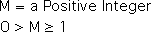
23. There are 2 necessary preconditions in the above equation and they both have to do with the nature of M, the Iteration Factor.
M = A Positive Integer
1) M must be an integer due to the iterative nature of the Living Algorithm's digestion process. M represents how many times the process has been iterated (repeated). The process is either performed or not. There are no partial processes.
2) M must be a positive integer for the algebraic expression to yield an Influence. This means that M must be 1 or greater, i.e. not negative and not zero.
Why for the 2nd condition? To facilitate comprehension let's talk a little about M's innate nature.
M = Number of Moments and the Number of Scalings
Notice that M serves two functions in the General Equation for Influences in the Living Average Grid (Equation 22).
1) When M is on the left of the expression, M indicates how many moments have passed in the Event since the initial Impact (how many iterations of the Living Algorithm process). In other words, when M is 1, only 1 moment has passed since the Impact. This is the 1st Influence. As M gets larger (2, 3, 4, …), the equation defines the size of the subsequent Influences. Accordingly, the General Equation precisely determines the value of all Influences in an Event when M is 1 or greater (M ≥ 1).
2) On the right of the equation, M is the exponent for K, the Scaling Factor. As the exponent, M determines how many times the original Impact has been scaled. Accordingly, the general equation indicates a simple relationship between Present and Future Influences. The Current Influence is multiplied (scaled) by K to determine the Next Influence. How simple! How elegant! The Present yields to the Future via a basic scaling process.
The General Expression for Impacts & Influences in the Living Average Grid
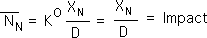
24. What happens to the general equation when M = 0? In other words, what happens when the expression is not scaled at all?

25. When M = 0, we are back to the beginning of the Event (NN bar). The Event is not scaled (K0 = 1) and we have the General Equation for an Impact.
26. If M is 0 or greater, rather than being exclusively positive, we can combine the General Equations for Impacts and Influences (Equations 22 and 25).

27. This slight change provides us with the General Equation for all the values of any Event in the Living Average Grid at any Moment, both Impacts and Influences.
This general equation determines the value of any member of any Living Average Event. Each member of the Living Average Event is a quantum of info energy. As such, this is the content-based equation that determines height of every info quantum (the colored rectangles) in our Living Average Grid. This is the equation we were looking for.
28. The values of the Events at the individual moments add up to yield the total Living Average at any moment in time. But the Living Average Events do not interact in any way whatsoever. Accordingly our general equation for the Living Average is also the general equation for the summation of Events. In other words, the terms in the general equation correspond with the info quanta for the Living Average. To illustrate, we show the data stream's 3rd Living Average as an example.
In other words the first term is the impact of Event C (no scaling – M = 0). In the 2nd term, Event B has been scaled once (M = 1). In the 3rd term, Event A has been scaled twice (M = 2).
Implications
What are the implications of this intriguing equation? The process is identical for every Living Average Event no matter when the new data point, XN, enters the System. The Event's first info quanta equals the Raw Data divided by D. We multiply this value, the value of the 1st quanta, by K to determine the 2nd quanta. We multiply the 2nd quanta by K to obtain the 3rd quanta, the 3rd quanta scaled by K to obtain the 4th quanta, and so forth.
The values of the quanta of each Living Average Event are totally independent of every other Event. There is no interaction between Events. No matter when the Raw Data enters the System, the process is identical. No matter what point in the cycle, no matter what the values of the surrounding data, the string of numbers that characterize the Event are solely determined by the initial Raw Data that spawned the event and its position in the stream.
As we shall see, this cozy relationship is not true for the Living Algorithm's higher derivatives – for instance, the Active Pulse's Directional. We shall examine the details in the next article in this series – Directional Quanta. But first, let us sink to a deeper level of understanding regarding our algebraic constructs – Impacts and Influences.
Present Moment = Instant’s Impact + Influences from Past Moments
The following section attempts to come to a deeper understanding of the relationship between the Living Algorithm, Impacts, Influences and Time, specifically the Past, Present, and Future. The following discussion is important because it will elucidate both our prior proofs and the proofs to come. Hopefully this mental exercise will warm the mind up so that it is flexible enough to embrace new constructs. Further, and perhaps more importantly, the analysis will reveal the fundamental nature of the Living Algorithm.
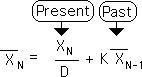
The Living Average = the Present + the Past
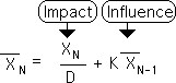
29. The Living Algorithm for the Living Average consists of 2 components. The sum of these 2 components yields the current Living Average, XN bar. The 1st component represents the contribution of the most recent data byte, XN, to the Living Average, XN bar. The 2nd component yields the contribution of past data bytes to the Living Average. Accordingly, the 1st component is associated with the Impact of the Present Instant and the 2nd with the Influences from Past Moments (shown below).
Remember that the Living Algorithm transforms Instants into Moments. In other words, the Living Algorithm digests Raw Data to create Data Stream Derivatives – such as the Living Average. Accordingly the Impact comes from the Raw Data of the Instant. The Impact produces an effect upon the individual Moment’s Composite Measures (such as the Living Average).
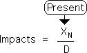
Impacts have no Past. Impacts correspond with the 1st component - contributions from the Present Instant.
30. This differentiation in the algebraic expression is reflected in our definitions of Impacts and Influences. For instance, Impacts have no Past. By definition, they institute the beginning of an Event. As the beginning there are no prior influences on the Impact. It just is.

31. In this case, the Living Algorithm's Past component (the 2nd) equals zero and drops out of the equation. Accordingly, the Living Algorithm's Present component (the 1st) equals the Impact of the New Data Byte, XN, on the Living Average. This whole package is associated with the contribution of the Present Instant to the Present Moment. This crucial point is where the external world exerts an Impact upon the dynamics of a data stream.
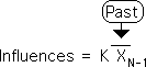
Influences have no Present. Influences correspond with the 2nd component - contributions from the Past.
32. Just as Impacts have no relationship with the Past, Influences have no relationship to the Present. By definition, Events are isolated from other Events. After a single Data Byte initiates an Event, no further changes occur. The partial system is allowed to run its course.

33. Because the Present doesn't exist for Influences, the 1st (Present) component drops out of the Living Algorithm. Only the 2nd (Past) component remains. Accordingly, the 2nd component of the Living Algorithm is associated with the Influences of Past Moments upon Present Moments.
The Living Algorithm: The Present Moment = the Impact of the Instant + Past Influences
34. The Living Algorithm's components combine to yield the Living Average at any moment. The Impact of the Instant combines with Influences that originated in the Past to generate the Present Moment.
Change and Residuals
Let us summarize and extend our analysis as a way of pointing to the next level of proofs - those regarding the Directional, the Living Algorithm's 2nd derivative. The Impact of the Instant, the Living Algorithm's 1st component, is associated with External Change. The Influence of Past Moments, the Living Algorithm's 2nd component, is associated with residual info energy. In other words, the Impact is the Change and the Influences are the Residuals from the Change. The rock splashes into the pond creating ripples on the surface. Keeping these basic bifurcations in mind will assist in understanding the proofs that follow.
Link
Thus far, our exploration of info quanta has yielded sheer simplicity. In other words, one elegant equation produces the values for every quanta of info energy in the Living Average Grid. This tidy relationship does not persist for the Directional, the acceleration of a data stream, the Living Algorithm's 2nd derivative. For details, check out the next article in this series – Directional Quanta.